Part 3 - How do I choose a KNN algorithm?
Part 3 in the Search and recommendations with embeddings series.
There are multiple algorithms to compute KNN, including both "Exact KNN" and Approximate Nearest Neighbors (ANN). When choosing between them, there is a tradeoff of quality for speed.
The Brute Force Approach - "Exact KNN" - O(N)
The simplest nearest neighbor approach is a Brute Force "Exact KNN" which takes O(N) time. To retrieve the K-Nearest Neighbors, the brute force approach is to compute the distances between your basis vector and all other vectors, sort them, and then choose the top K.
For example, to find the KNN of an Unknown Animal and 10 million animal embeddings, you would have to do 10 million distance calculations, sort the distances from nearest to farthest, then take the top K. Our performance testing measured that a dot product between two 50-Dimensionsal vectors, with the data already in memory, on an AWS i3.4xlarge 2.3 GHz processor, takes on average 100 nanoseconds. So to find song recommendations for a customer from 10 Million possible tracks would take 1 second of CPU time (100 nanos * 10 M = 1 second) to do just the math on a single processor.
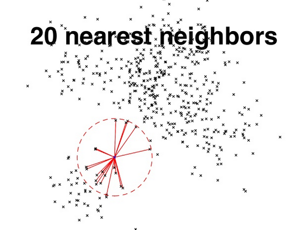
Computing distance to each vector to see who nearest neighbors (less efficient, best recall)
The problem is, customers are very sensitive to speed, and a 1 second time to get a response can be disastrous. Amazon famously found every 100ms (0.1 seconds) of latency cost them 1% in sales. Google found an extra 500ms of latency in search page generation time dropped traffic by 20%.
Faster than Brute Force?
With high dimensionality, and lots of entities, a Brute Force gets even worse. So researchers have come up with faster algorithms than Brute Force "Exact KNN". These alternative algorithms make a quality for latency trade-off, where the set of nearest neighbors calculated is not always exactly equivalent to the “Exact KNN” approach, and hence, these algorithms are refered to as “Approximate Nearest Neighbors” (ANN).
ANN - Approximate Nearest Neighbors - O(log n)
Approximate Nearest Neighbor algorithms finds probably the nearest neighbors, but not guaranteed. With ANN algorithmss, the closer to recalling perfect nearest neighbors (the exact KNN result) the slower the search (you have to do more comparisons and get closer to Brute Force).
There are different algorithms to do ANN, each with its own performance/recall trade off curve. Here is a subset of them below.
Algorithm 1 - annoy
One algorithm to reduce the number of comparisons you have to do, is to repackage the vectors into hierarchical trees, e.g. R-trees, you can compare your vector to the split criteria, rather than all points. This means you can find nearest neighbors in logarithmic time instead.

To explain what that means visually, one ANN algorithm, annoy can be explained with pictures. Annoy (Approximate Nearest Neighbors Oh Yeah) was developed at Spotify, and powers their recommendations. (source: https://www.slideshare.net/erikbern/approximate-nearest-neighbor-methods-and-vector-models-nyc-ml-meetup ):
Split the vector space with hyperplanes to reduce the number of comparisons you have to do. Rather than computing distance to a particular point, you compute which side of a hyper plane you are on, and look for nearest neighbors in that space, for each subspace.
- Am I above/below the middle bold line.
- Okay, I’m above, that puts me in the green or orange territory...next, am I left or right of the next split (am I in orange or green area)
- splits continue, etc..
- Find bottom, nearest neighbors are ones in the same space
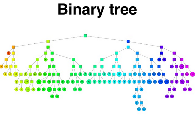
This is the data structure that gets built, where to decide to go down left of right branch, you are comparing to the pivot criteria (am I above/below a hyper plane).
Once you have descended all the way down to the leaf nodes, you have found your approximate nearest neighbors.
Algorithm 2 - Hierarchical Navigable Small World (HNSW)
There is an implementation of HNSW called Non-Metric Space Library (NMSLIB). It is more efficient than the “annoy” approach described above. Rather than splitting into trees, it hops around in vector space, from sub-graph to sub-graph, from vector to vector, greedily choosing the next nearest point until it descends close to the target. It is more efficient than the approach of annoy.
The Amazon Elasticsearch team wrote an Open Distro plugin to make HNSW-NMSLIB run on Elasticsearch. Written about here.
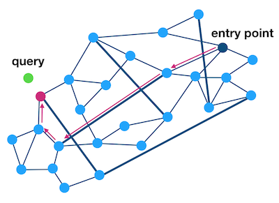
The algorithm starts by choosing a point at random, computing its distance to the target (query).
Then proceed to explore the graph, by continuing to choose the next closest point (based on Euclidean distance), until you find no closer points.
The graphs are built as a hierarchy of smaller graphs, so you start at a coarse layer (small subset of points), finding the nearest sub graphs, then you navigate those sub graphs.
Choosing an ANN Algorithm
ANN-Benchmarks is a benchmarking environment for approximate nearest neighbor algorithms search.
Spotify uses annoy for recommendations. in graph below, dark blue line
- Algorithm used: Annoy uses the approach described above
Amazon Elasticsearch KNN Service uses hnsw (nmslib). in graph below, light blue line
- Algorithm used: The HNSW (NMSLIB)
- For 80% recall, the benchmark below suggests we can reach ~3000 TPS, for ~95% recall, 500 TPS
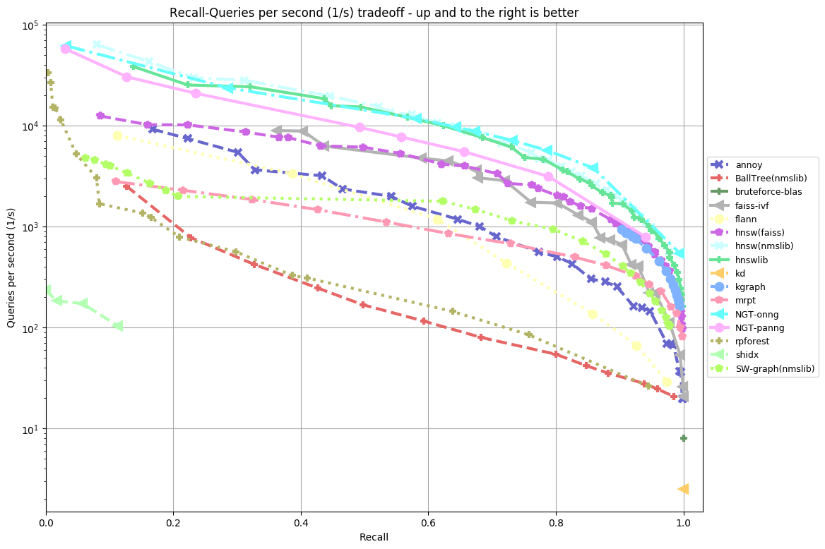
( source : http://ann-benchmarks.com )